LeRoPE: letting RoPE learn its own frequencies
With Mistral Large 4 adopting LeRoPE, we figured it was a good time to write about it. LeRoPE makes RoPE’s rotation frequencies learnable, along with the rest of the network.
This post is an overview of the method and what we found. If you only want to try it, skip to the code.
TL;DR: 32 parameters → 3.4% less pretraining compute.
- LeRoPE learns one scale per RoPE frequency. That’s \(d_h/2\) extra parameters, a few lines of code, and no meaningful compute overhead.
- Across 176 pretrained models from 52M to 2.5B parameters, it beats both RoPE and p-RoPE at every scale. It saves 3.4% of pretraining compute at 2.5B as well as improving long-context retrieval.
- We found that generally fast rotations track RoPE, rotations slower than the training context get shut off, and one channel ends up carrying almost all the positional signal.
- If you pretrain a model with RoPE, it’s essentially free.
RoPE
RoPE rotates the queries and keys in attention according to their position in the sequence. Each 2-dimensional chunk (or channel) of a query or key rotates at its own fixed frequency, and the frequencies follow a geometric schedule set by a single hyperparameter, the base \(b\):
\[\theta_m = b^{-2m/d_h}, \qquad m = 0, \dots, d_h/2 - 1.\]Because the rotations compose, the attention logit splits into one term per channel, and each term depends only on how far apart the query and key are. With 64-dimensional heads and the default \(b = 10{,}000\), the channels’ wavelengths (\(2\pi/\theta_m\)) run from about 6 tokens to about 47,000. In a 2,048-token context, the slowest 11 of the 32 channels never complete a single turn.
Prior work has found some benefit to having stable channels that don’t rotate (or at least not much). They’re useful for long-range semantic information, where the exact relative position doesn’t matter. So in practice people now either scale up \(b\), don’t rotate the slowest channels (p-RoPE), or don’t apply RoPE altogether (NoPE). All of these help, but all of them pick the frequencies by hand. We wanted to see what the model would choose for itself.
LeRoPE
The method is one line:
\[\hat\theta_m = e^{\alpha_m}\,\theta_m ,\]
with one learned \(\alpha_m\) per channel, shared across all layers and heads, and initialized at zero so the model starts out as plain RoPE. Some practical notes from our experiments:
- Clip the frequency gradient separately. The gradient of the frequency grows with the context length. If it shares a clipping norm with the rest of the model, it dominates that norm. We found clipping the LeRoPE parameters separately led to stable training.
- No weight decay on \(\alpha\), which is less of a prior on RoPE.
- Learn it in log space. We found this to have better optimization dynamics than directly learning the frequency or learning linear scales.
- Only one set of scales is needed. Learning separate scales per layer or per head did not improve performance and cost extra parameters.
Results
To validate our method we trained a ladder of models ranging from 52M to 2.52B. All models were trained with 20 tokens per parameter on C4 at sequence length 2,048. Here’s validation perplexity:
| Method | 52M | 217M | 608M | 1.34B | 2.52B |
|---|---|---|---|---|---|
| RoPE | 30.2450 | 18.2377 | 13.8795 | 11.5747 | 10.1720 |
| p-RoPE | 30.2695 | 18.2269 | 13.8663 | 11.5665 | 10.1659 |
| LeRoPE | 29.9479 | 18.1335 | 13.8093 | 11.5384 | 10.1387 |
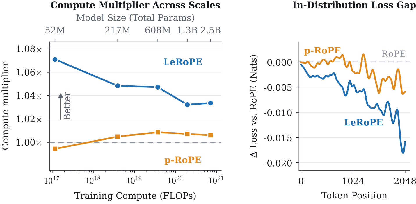
LeRoPE is 3.4% more compute efficient than RoPE at our largest scale and its gains grow over the context length suggesting better context utilization. In the paper, we also include multi-seed evaluations as well as another scaling ladder trained on StarCoder data. LeRoPE remains a winner in these too.
Long context
The real gains from LeRoPE show up in long context tasks. We evaluate our 2.52B models with YaRN on RULER’s 8 needle-in-a-haystack tasks and include a 2.52B model trained with a base frequency of 500k.
| Mean accuracy, 8 NIAH tasks | 2K | 4K | 8K | 16K | 32K |
|---|---|---|---|---|---|
| RoPE | 0.509 | 0.457 | 0.351 | 0.245 | 0.152 |
| RoPE, base 500k | 0.543 | 0.493 | 0.420 | 0.286 | 0.159 |
| p-RoPE | 0.548 | 0.498 | 0.398 | 0.238 | 0.146 |
| LeRoPE | 0.608 | 0.573 | 0.511 | 0.390 | 0.214 |
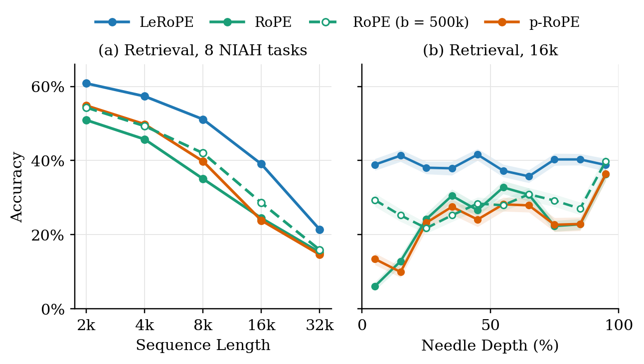
At 16K, LeRoPE’s accuracy is roughly flat across needle depth, while RoPE and p-RoPE collapse for needles near the start of the context. The larger base fixes that collapse but otherwise stays near RoPE.
What frequencies do we learn?
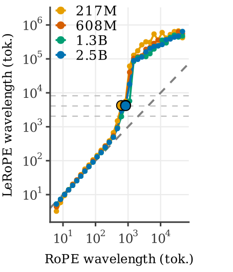
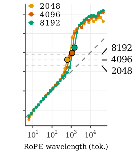
The learned pattern is the same across scales and seeds. Fast rotations track standard RoPE (the fastest even speed up a little). Rotations slower than the training context get shut off almost entirely. Where that cutoff falls moves with the training length (right panel).
So is LeRoPE just a learned p-RoPE? Not quite. LeRoPE’s cutoff lands around channel 17 of 32, which is roughly p-RoPE with \(p = 0.5\). But p-RoPE cut there does no better than the standard \(p = 0.75\), so the cutoff alone isn’t where the gain comes from. It comes from how LeRoPE reshapes the channels it keeps, which no choice of \(p\) can express.
One dominant positional band
Since the logit splits by channel, we can look at each channel’s contribution as a function of offset. In LeRoPE models, one channel takes over the positional work almost completely. We call it the dominant positional band:
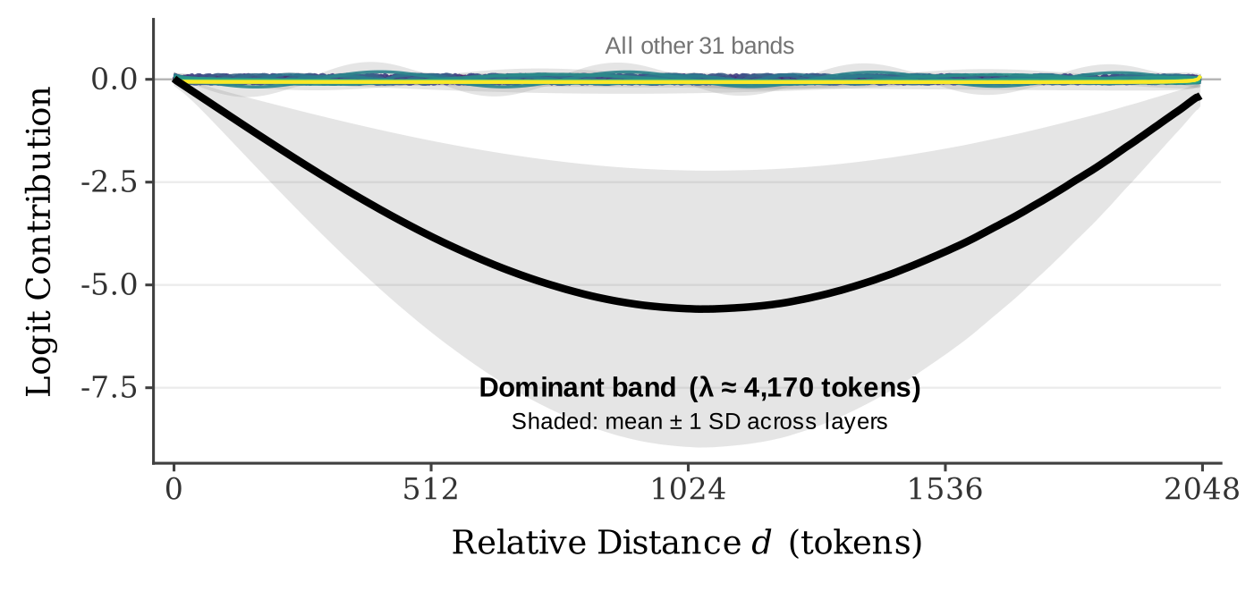
It’s channel 17 in our 608M to 2.5B models (16 at 217M). LeRoPE slows it about fivefold, to a wavelength a bit over twice the training length (2.0–2.3× across six runs). So across the training window it traces roughly half a period. Zero at offset 0, most negative mid-window, and back near zero at the edge. It acts as a fairly consistent relative positional bias. The model relies heavily on it. Zeroing this one channel raises the loss by 0.76 nats while no other channel costs more than 0.07. RoPE and p-RoPE don’t show anything close to this level of consolidation.
We worried that a bias like this would make LeRoPE ignore medium- and long-range dependencies. It doesn’t. As the results above show, LeRoPE’s gain over RoPE actually grows with position in the context.
One more question: is the gain about the frequencies LeRoPE finds, or about learning them? It seems to be both. Training a fresh model with LeRoPE’s learned frequencies frozen recovers only about two thirds of the gain (63.6%; p-RoPE recovers about a tenth). The full gain needs the frequencies and the rest of the weights to co-adapt during training.
Trying it yourself
Here’s a minimal PyTorch version. It uses interleaved pairs, dims \((2m, 2m{+}1)\), as in the paper. If your codebase pairs dims \(m\) and \(m + d_h/2\) instead, keep its convention: only the frequencies change.
import torch
import torch.nn as nn


class LeRoPE(nn.Module):
    """RoPE with one learned log-scale per frequency band.

    Create one instance per model and share it across every attention layer.
    """

    def __init__(self, head_dim: int, base: float = 10_000.0):
        super().__init__()
        m = torch.arange(head_dim // 2, dtype=torch.float32)
        self.register_buffer("theta", base ** (-2 * m / head_dim), persistent=False)
        self.log_scale = nn.Parameter(torch.zeros(head_dim // 2))  # alpha_m; zeros = RoPE

    def forward(self, x: torch.Tensor, pos: torch.Tensor) -> torch.Tensor:
        # x: (batch, heads, seq, head_dim); pos: (seq,) token positions
        freqs = self.theta * self.log_scale.exp()             # (head_dim/2,)
        angle = pos.float()[:, None] * freqs[None, :]         # (seq, head_dim/2), fp32
        cos, sin = angle.cos(), angle.sin()
        x1, x2 = x[..., 0::2].float(), x[..., 1::2].float()   # band m = dims (2m, 2m+1)
        out = torch.stack((x1 * cos - x2 * sin, x1 * sin + x2 * cos), dim=-1)
        return out.flatten(-2).type_as(x)
Apply it to both queries and keys, as with RoPE. Then set up the optimizer with the clipping and weight-decay notes from above:
freq_params = [model.rope.log_scale]
other_params = [p for p in model.parameters() if p is not model.rope.log_scale]

opt = torch.optim.AdamW(
    [{"params": other_params, "weight_decay": weight_decay},  # keep your usual no-decay groups
     {"params": freq_params, "weight_decay": 0.0}],
    lr=lr, betas=(0.9, 0.95),
)

# each step, after loss.backward():
torch.nn.utils.clip_grad_norm_(other_params, 1.0) # if you're using gradient clipping
torch.nn.utils.clip_grad_norm_(freq_params, 1.0)  # its own norm
opt.step()
Also we compute the angles in fp32, and use a scaling method such as YaRN if you run past the training length. If you’re pretraining with RoPE or p-RoPE, this is essentially free, so give it a try!
This was joint work with Shreyas Kadekodi, Rui Zhu and our advisor Julian McAuley. We’re always happy to chat! The easiest way to reach us is by email (pkarypis [at] ucsd [dot] edu and seobrien [at] ucsd [dot] edu) or on X (@kpetro_research and @seano_research).
@article{karypis2026lerope,
  title   = {LeRoPE: Learnable RoPE Frequencies Improve Language Modeling},
  author  = {Karypis, Petros and O'Brien, Sean and Kadekodi, Shreyas and Zhu, Rui and McAuley, Julian},
  journal = {arXiv preprint arXiv:2607.10134},
  year    = {2026}
}